LARE-HPA
Summary
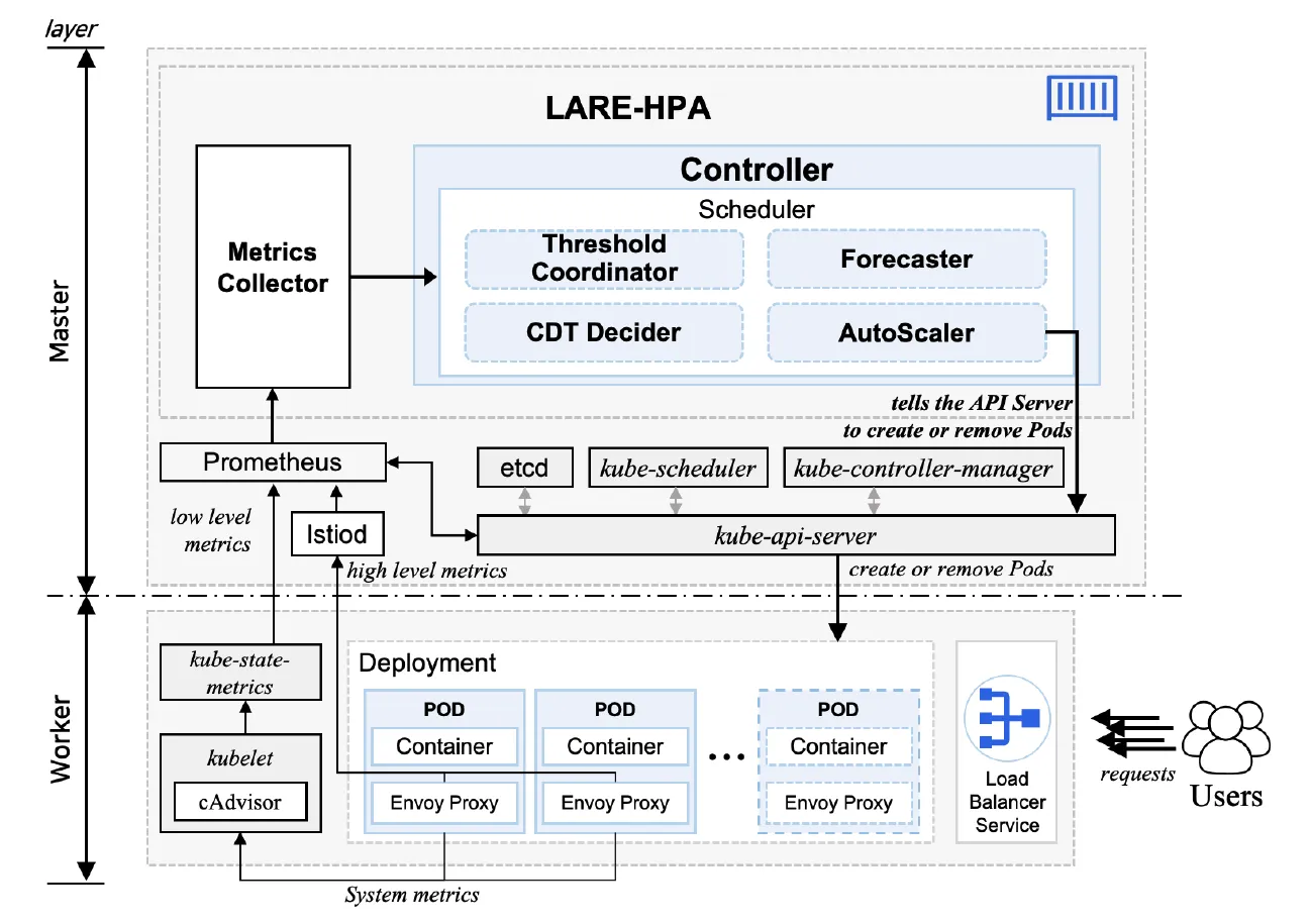
A Kubernetes autoscaler that adjusts the CPU Threshold and Cool Down Time as requests change. I designed and implemented a Python controller that updates request forecasts without separate offline training and coordinates when to scale out and release resources.
- Role
- First Author (method design and implementation, experiments)
- Stack
- Python, Kubernetes, Istio, Prometheus
- Outcome
- ICSOC 2024 Distinguished Paper Award, patent application filed, software copyright registered
Problem
Load Changed, but the Scaling Criteria Stayed Fixed
Kubernetes’ built-in HPA adjusts replica counts by comparing CPU utilization with a configured Threshold. A lower Threshold can prepare replicas earlier and reduce latency, but requires more resources for the same requests. A higher value uses more of each replica, yet requests can queue while new replicas become ready. Balancing latency and resource efficiency called for criteria that could change with the load.
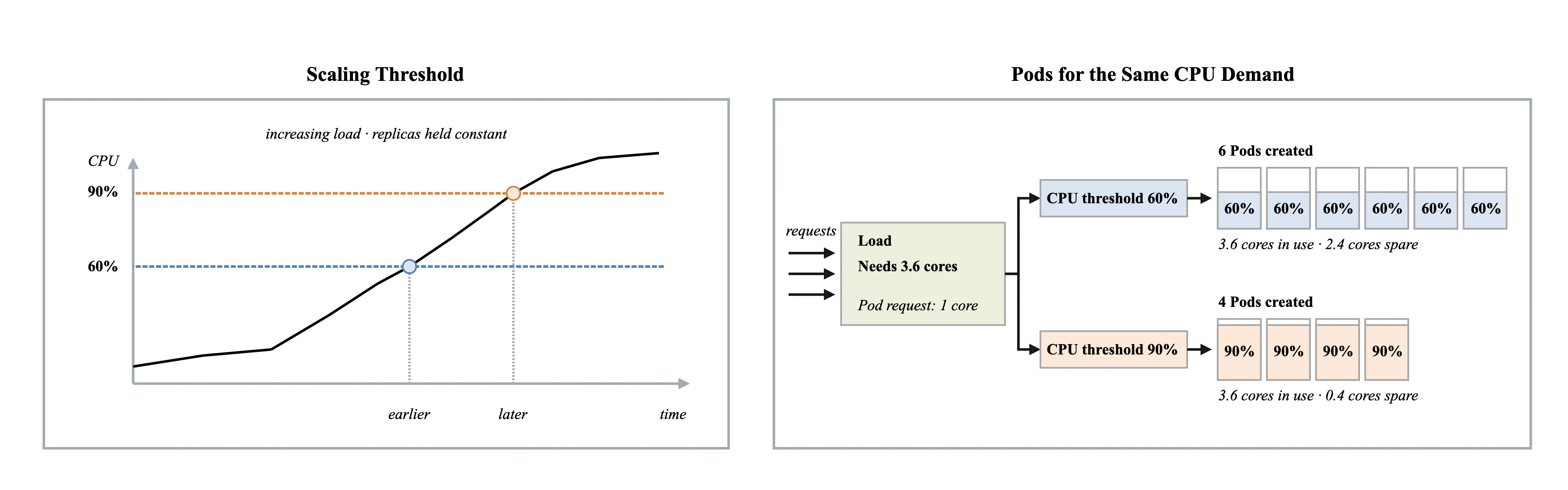
I first compared different Threshold settings. Mean CPU allocation was 1,280.0 millicores at 60% and 1,046.15 millicores at 90%, a difference of about 22%. This comparison exposed the cost of applying one setting across stable and rapidly changing periods.
The timing of scale-in presented a related problem. A short Cool Down Time can cause flapping when replicas released after a brief dip must soon be added again. A long value retains resources after demand has fallen. The headroom for scaling out and the wait before scaling in needed separate adjustments as requests changed.
Design Direction
Learning from Incoming Requests Without Waiting for Offline Training
Adjusting the criteria required information about how requests were changing alongside current CPU utilization. New applications have little history for training, and a previously trained model may need retraining when request patterns change. I chose online learning to keep updating forecasts from data collected during execution.
The Forecaster uses Online ARIMA. An online autoregressive approximation represents the relationships between past observations and errors, and Online Newton-Step updates its coefficients as observations arrive. This provides a forecast for the next interval without repeating a separate offline training stage.
Forecasts and observed request changes feed the Threshold adjustment. Current CPU utilization and the adjusted Threshold determine the actual replica count. The controller retains the configured Threshold while initial observations accumulate, then starts applying adjustments once the forecasting model is ready.
Design #1
Bringing Scale-out Forward When Requests Become More Volatile
The same increase in requests can mean different things depending on normal traffic volume and variation. I designed the Threshold Coordinator to compare recent request changes and the next forecast with the application’s historical level of volatility.
A z-score standardizes the recent change level using the last 10 intervals and the forecast. An inverse sigmoid then maps it into a CPU Threshold range. This turns an unbounded request count into a value the CPU-based scaling decision can use. The experiment used a range of 50–95%.
Higher volatility lowers the Threshold to prepare resources earlier; lower volatility raises it to use existing replicas more fully. The criteria can therefore differ at the same request volume as the recent pattern changes. Combining forecasts with observations also carries actual changes into the next decision.
Design #2
Keeping a Brief Dip from Releasing Replicas Too Soon
The Threshold changes when to scale out, while Cool Down Time controls when resources can be released. During an overall rise in demand, a brief dip calls for waiting. During a decline, unnecessary replicas should be released sooner.
The CDT Decider fits a linear regression to the 60 most recent observations to identify the direction of demand. It also checks the residuals, the differences between observations and the fitted line, with the Durbin-Watson statistic. A trend affects the target waiting counter only when residual autocorrelation meets the configured acceptance range: an upward direction lengthens the wait and a downward direction shortens it.
Waiting is counted in metric-collection cycles. I kept the target wait separate from the remaining counter and decremented the latter each cycle. Scale-in is allowed only when that counter has expired and the CDT Decider does not return an upward direction. Scale-out can be requested whenever more replicas are needed, regardless of the waiting counter.
Implementation
Connecting the Adjusted Criteria to Kubernetes Scaling
I implemented the two adjustment paths in a Python controller that changes actual replica counts. Inside one Pod, request forecasting and Threshold adjustment, Cool Down Time adjustment, and scaling run as three asynchronous processes. Shared locks protect reads and updates to the adjustment values.
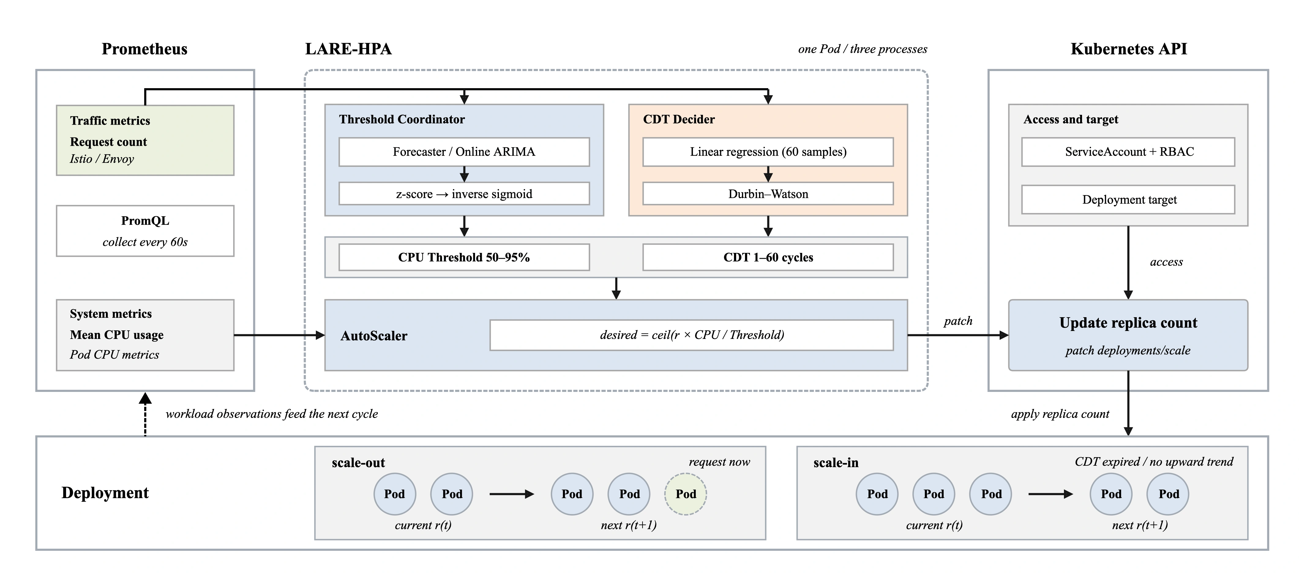
The controller periodically queries system metrics and Istio request metrics in Prometheus. The AutoScaler rounds up current replicas multiplied by average CPU utilization divided by the adjusted Threshold, then applies the configured replica limits. It checks scale-out or scale-in conditions and updates Deployment replicas through the Kubernetes API.
The controller runs as a container separate from the application. A ConfigMap specifies the target application, Prometheus endpoint, initial Threshold, replica limits, and collection interval. A ServiceAccount and RBAC provide API access. Operating independently of the target application allows the controller to be applied to different applications without changes to their code.
Logs record forecast requests, the Threshold, Cool Down Time, scaling decisions, and errors. These records connect a change in replica count to the observations and criteria that produced it.
Evaluation and Results
Comparing Latency and Allocation on the Same Request History
I replayed NASA-HTTP requests against a PHP application that computes trigonometric functions, using master and worker hardware with an Intel Core i9-10900K and 32 GiB of memory. With a one-second response-time SLO, I compared latency and the proportion of requests meeting the target, including periods of abrupt demand changes.
The baselines were default HPA, offline-trained Bi-LSTM, and Online-BO based on online Bayesian optimization. Bi-LSTM was trained on 50% of the workload with a per-Pod request-handling limit of 50. LARE-HPA used 10 intervals for Threshold coordination and 60 for CDT decisions; the other baselines followed their original papers’ configurations. These comparisons covered fixed settings, offline learning, and online optimization.
LARE-HPA achieved the lowest mean latency and highest SLO attainment among the four methods in this experiment. Mean latency fell from 562.8ms with default HPA to 279.5ms, a 50.34% reduction, while P95 fell from 1,189.0ms to 600.1ms. SLO attainment rose from 93.86% to 97.24%, an increase of 3.38 percentage points.
| Method | Mean Latency (ms) | P95 Latency (ms) | Mean CPU Allocation (millicores) | SLO Attainment (%) |
|---|---|---|---|---|
| HPA | 562.8 | 1189.0 | 582.76 | 93.86 |
| LARE-HPA | 279.5 | 600.1 | 638.13 | 97.24 |
| Bi-LSTM | 462.1 | 1062.6 | 875.85 | 93.06 |
| Online-BO | 519.3 | 966.3 | 1274.75 | 95.15 |
Abrupt request increases also exposed differences in how the baselines responded. Bi-LSTM did not provision enough replicas when demand exceeded its learned patterns. Online-BO also had intervals where rising demand was not addressed before P90 latency exceeded twice P50 latency, its adjustment trigger. These observations reinforced the need to adjust the Threshold as requests change and retain replicas during an upward trend.
I interpreted CPU allocation alongside latency. Default HPA allocated the least CPU; LARE-HPA used more resources while improving latency and SLO attainment. It achieved the lowest mean latency with less mean CPU allocation than either learning or optimization baseline, showing the resulting balance between response performance and allocation.
Research Outcomes
Turning Fixed Settings into Rules Updated from Observations
The central lesson was to design the scale-out and scale-in decisions separately. Headroom for abrupt changes and time to wait through a brief dip address different problems. I used volatility and trend as inputs to those decisions and jointly optimized latency and resource allocation.
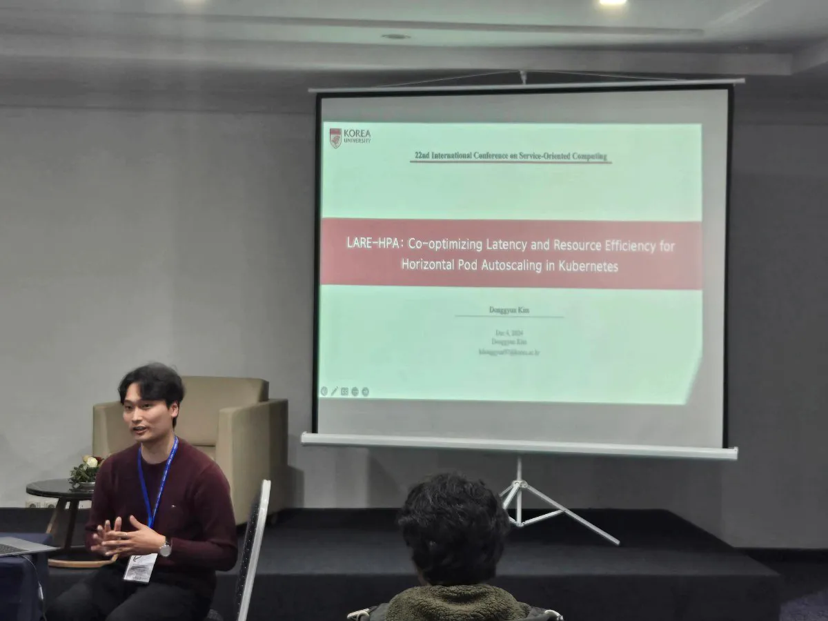
The study was published at ICSOC 2024 and received a Distinguished Paper Award. I presented LARE-HPA’s design and experimental results at the conference in Tunis, Tunisia, in December 2024.
A patent application (10-2024-0128875) was filed, software copyright (C-2024-043831) was registered, and the implementation was released as open source.
The equations and full experimental configuration are available in the published paper.